Implementing overlapping date-range queries in Kube

Warning: this post is about me experimenting and researching on the subject, I am not an authority in the matter.

I want my calendar view to be optimized, how hard can it be?

To be more precise, I want the events displayed in a calendar view (week view, month view, etc.) to be fetched quickly from the database, without having to load them all into memory, while not overblowing the size of the database. Some people use their calendar extensively and we do not want to make Kube memory or disk heavy for them.

In Kube, we’re using LMDB as a database. Think of it as a low-level, embedded, key-value database. LMDB uses B-Trees as internal data structures. From the API side, we can jump to a given key, jump to an element whose key is greater or equal than a given, and many other wonderful things.

Naive search

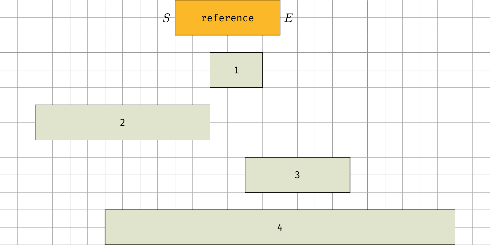
Case 2–4 shows that the starting time of the event can be anywhere before the ending time of the reference period. Conversely, the ending time of the event can be anywhere after the starting time of the reference period.

In the naive case, where we only have a table containing events, this means that we have to go through every element and filter according to their periods.

Search in sorted index

A somewhat obvious optimization is to use two sorted indexes: one for the starting time of events, and one for ending times.

A sorted index would look like this:

DateTime	Reference
2018-06-20 13:45:00	Event 1
2018-06-20 13:45:00	Event 2
2018-06-20 14:00:00	Event 3
2018-06-21 09:30:00	Event 4

The “Reference” column only contains the “id” of the event in the “Events” table, so that we can fetch it later, if needed.

If we have both sorted indexes (starting and ending times), then we could fetch the intersection of the set of events whose starting time is from the start of the dataset until S, and the set of events whose ending time is from E, until the end of the dataset.

Even though we still have to go through all events in the indexes (with some duplicates), it should still be better for a big dataset because:

• Going through the index is faster than the original dataset
• Going through the index consume much less memory than with the original dataset
• But, more disk space is required

But still, I think we can do much better.

Quick analysis

One way to really optimize is to find a way to know, given a query, where events would be in the dataset, either by ordering them clevery (better for caching), or by having a mapping function (still much better than the naive search).

What we could do is to index both starting and ending times of the event using a two-dimensional index.

Since it’s a search in 2D space, let’s plot some graphs:

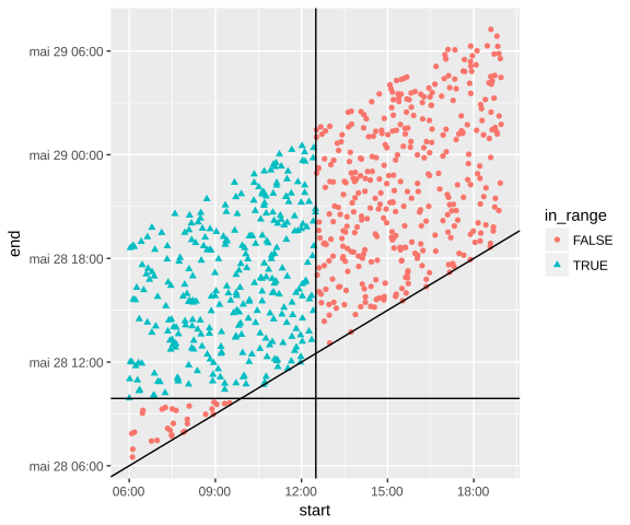
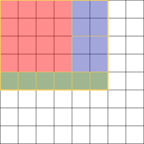
In the first figure, we see that periods that overlaps with a given range are all cranked up in an upper left square. This can be explained by the condition:
a period A overlaps with another period B if and only if:

A[start] ≤ B[end] and B[start] ≤ A[end]

From this, we can deduce the bounding box of the events in figure 18: the horizontal line is Ref[start] and the vertical line is Ref[end].

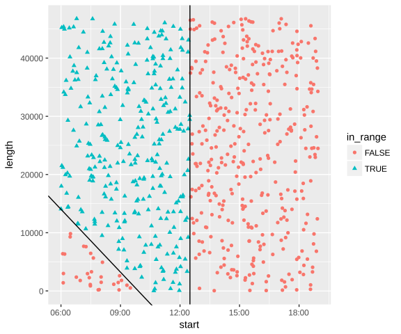
For the second figure, we can deduce the slanted line by changing part of the equation above, and we get:

-x + Ref[start] ≤ y

Searching in a somewhat arbitrary quadrilateral might seem harder than a square, probably because it is. But since the search heavily depends on the way we store periods in the index, who knows?

Now that we know which search we have to do, we have to find a method of storing discrete two-dimensional data in one dimension while preserving the most “locality” possible: since the interesting events are in the same “area” in both representations, the closer they are in the index, the more we can find them in batches, the more optimized it will be.

Space-filling curves

The first method we can use to store multi-dimensional data is using space-filling curve. It can also be thought as surjective function that maps a one dimensional coordinate to n-dimensional coordinates.

What we do is we use the inverse function of the space-filling curve, pass our multi-dimensional data as argument which gives us a single number. We can then use this number in an sorted index, which will map to a reference in the event table.

One example of this kind of curve is the Hilbert Curve.

A very nice explanation on how to use the Hilbert curve to transform two-dimensional data to one-dimensional and back has been made by Grant Sanderson on the 3Blue1Brown YouTube channel.

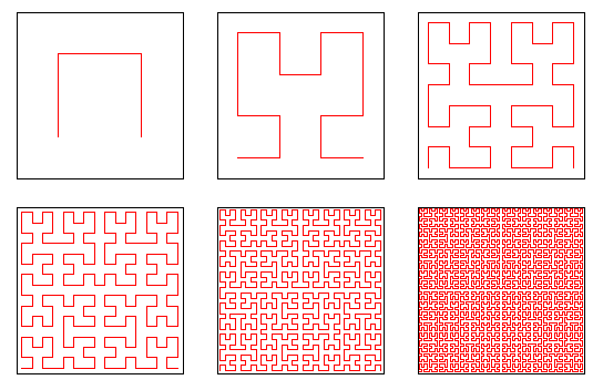
Credit: Dr Fiedorowicz — https://commons.wikimedia.org/wiki/File:Hilbert_curve.png

This figure represents different orders of the Hilbert curve. We can also think of it as different zoom levels: in the top-left figure, the curve goes through 2×2 pixels, top-middle figure 4×4 pixels, top-right 8×8 pixels, etc.

However, while this is a well-known curve and preserves fairly well locality, this might not be the most adapted: if we index according to event starting times and ending times, since events never end before they start, at least half of the curve will end up unused.

But we can find triangular space-filling curves: meet the Peano curve:

Credit: Peano curve. Encyclopedia of Mathematics. — http://www.encyclopediaofmath.org/index.php?title=Peano_curve&oldid=32355This curve perfectly maps or input domain (squared triangle) and seems to also preserve locality well.

In practice, here’s how it would work:

We need to know:

• f^-1: x, y -> i To index elements
• f: i -> (x, y) Will surely be used to get parts of the curve

Should someone want to search in a given period, the process would be:

1. Somehow get the bounds i_min and i_max such as i_min ≤ f^-1(x, y) ≤ i_max for all x and y in the search zone.
2. Go through every elements between i_min and i_max in the index, and filter the ones not in the search zone. The more the curve preserves locality, the less we will filter elements out.

Or

1. Somehow get the “batches” of the curves that overlaps with the search area.
2. Go through each of the batches in the index, and report every events associated. The more the curve preserves locality, the bigger the batches, the better.

All in all for our case, the criteria for a good space filling curve is that:

• Each segment goes through each pixels
• Maybe triangular
• Easy to get batches our bounding indexes of the curve
• Preserves the most locality for both 1D to 2D and 2D to 1D conversion

However, the 2D plot is misleading: in reality we will not have random events. Most events will not intersect and we will probably have no more than 5 events a day. This means that the data will be much more sparse. Hence, if we use the second method and have a lot of small “batches”, we will end up searching a lot of nothing.

Infinite binary trees

While messing around with the triangular Peano curve, I found an interesting way of storing data that resembles the H Tree, Quadtree.

We start with a small triangle, conceptually composed of 3 pixels at the bottom left of the graph. To each pixel, we associate a binary number: 00, 01, 10. Then you assign this triangle the digit 0, duplicate and mirror it above, and assign 1 to the new triangle. Then repeat this process.

Another way of looking at its construction is by subdividing the triangular 2D space by two recursively.

We now have a way of associating coordinates in a triangular 2D space to a single number: by concatenating digits, starting from bigger triangles to smaller triangles. What’s more is that if the numbering is coherent, we can grow these triangles indefinitely without having to change the numbering of the pixels.

Then if we need to search a subset of the data, we can somewhat easily use the visual representation to find ranges/batches where the data is interesting to us: since we now the binary prefix, we can easily deduce inequalities.

Otherwise the process is very similar to the one with space-filling curves.

After some searching, I found that the “Infinite Binary Tree” is very similar to Quadtrees. Quadtrees are the conventional square version: instead of splitting a triangle into 2 smaller triangles, you split a square into 4 smaller squares. By labelling 00, 01, 10 and 11 each squares, repeating the process and concatenating the labels, you can also convert 2D coordinates to 1D.

In our use case, the big advantage of Quadtrees against the “Infinite Binary Tree”, is that being a square, doing rectangular searches would be much simpler, and probably more optimized.

Also, as with the “Infinite Binary Tree”, the Quadtrees have its space-filling curve counterparts: by ordering the labels right, we can get exactly the same ordering as the Hilbert Curve or the Z curve.

Hence, we could use exactly the same method for indexing and retrieving events as for space-filling curves.

However, by looking and the quadtrees, we can find an interesting method of retrieving events:

• We can find the smallest power of 2 bounding the search area, and use post-filtering
• We can “rasterize” the search area and get exact batches of the curve, and not use post-filtering

The “rasterisation” would be something like this:

• let “res” be the empty set of resulting squares
• let “proc” be the empty set of squares to process
• Store the smallest power of 2 bounding the search area into “proc”
• While “proc” is not empty
  • Split the current square into 4
  • For each resulting square “s”
    • If search area overlaps with “s”
      • If “s” is contained in search area
        • Store “s” in “res”
      • Else add “s” to “proc”
• Return “res”

Even though this algorithm is nicely parallelizable using a “proc” as a thread pool, there can be a lot of squares to process, should the size of the search area be big. In our use case, most of the search will be on a recent week or month. That means if the dataset starts at 1970-01-01 00:00, the search area will be quite big for a week in July 2018 (at least horizontally).

Like with the “batches” method of space-filling curves, we shouldn’t subdivide the search space too much. But one advantage with this solution is that we can modify the algorithm to limit the number of recursions and apply post-filtering to avoid the problem.

Buckets

I have to confess first, this solution was not from me, but from Christian.

This solution uses the fact that we will want to search for every event within a week. We will just have an index that associate a given week (bucket) to a list of events that occurs within this week:

Week Number	Reference
42	Event 1
42	Event 2
42	Event 3
43	Event 3
44	Event 3
51	Event 4

We see that there are duplicate keys, but since LMDB uses B-trees internally, the key shouldn’t appear multiple times in the storage.

We can also see that events can span over multiple weeks. However in a normal dataset, there won’t be many events that will last over that much time: even though there are real-world cases (a party on Sunday that lasts after midnight, or a vacation over a couple of weeks), this probably won’t result in a massively oversized index.

In terms of performance, if we are fetching events in a given week we just have to calculate the week number, and return every event in this bucket.

If this is a month view, we do the same with multiple weeks.

For a generic search, we do the same and apply post-filtering.

This solution is by far the simplest and most elegant one. This follows that this is probably the fastest one, compared to space-filling curves and infinite
binary trees.

However this solution works only because we are working with ranges and not generic two-dimensional data.

But this is perfect for our use-case and so, this is the solution we are currently using.

Conclusion

I would have liked to spend some time benchmarking different curves and trees, but the solution we have is just too good.

There are so many things to consider and evaluate, I’m kinda lost.

I was beginning to forget a key thing: with have the luxury of knowing the form of the data we will have: mostly events with a timespan of a couple of hours. Some outliers may exist, but they are rare, and our solution better has to reflect that.

Graphics made with R (ggplot2), TikZ and Asymptote